1 LV Shape Atlas

The LV shape atlas was built by using Principal Component Analysis (PCA) on the concatenation of end-diastolic (ED) and end-systolic (ES) surface points. Let \(\mathbf{S}\in\mathbb{R}^{n\times 3m}\) be a shape matrix from \(n\) cases with \(m\) points in 3d Cartesian coordinates. Hence, each row \(\mathbf{s}_i\) in \(\mathbf{S}\) is a vector of \[ \mathbf{s}_i = \left[x_1, y_1, z_1, \ldots, x_m, y_m, z_m \right]^T\ \mathrm{for}\ i\in[0,n] \]

Let \(\mathbf{\mu}\in\mathbb{R}^{m}\) be a mean shape vector, \(\mathbf{\Phi}\in\mathbb{R}^{3m\times p}\) be the first \(p < n\) principal components, and \(\mathbf{B}\in\mathbb{R}^{n\times p}\) be the principal scores. The PCA linear relationship for the LV shape atlas is given by \[ \mathbf{S} = \mathbf{1}_n\ \mathbf{\mu}^T + \mathbf{B}^T\mathbf{\Phi} \]

Implementation note

The codes are written in Matlab language. LV shapes are derived from 3D finite element models defined in prolate spheroidal coordinate.

1.1 Mean shape estimation

function cc_mean = mean_shape(S, varargin)
% Align all shapes
nshapes = size(S,1);

% default values
opts.max_iter = 10;
opts.error_bound = 1e-16;
opts.mean_shape = NaN;

% get the options
for i=1:2:length(varargin)
    if isfield(opts, lower(varargin{i}))
        opts.(lower(varargin{i})) = varargin{i+1};
    else
        error('Unknown option %s', varargin{i});
    end
end

% get the mean shape to align
cc_mean = opts.mean_shape;
if isnan(cc_mean)
    % get random shape as the first mean
    cc_mean = S(randsample(nshapes, 1), :);
end

% start the iteration
finish = false;
iter = 0;
while ~finish && iter<opts.max_iter
    iter = iter + 1;

    % procrustes distance from each shape to the mean
    Pm = shape2points(cc_mean);
    for i=1:nshapes
    
        P = shape2points(S(i,:));
        [~, Z] = procrustes(Pm, P, 'reflection', false, 'scaling', false);
    
        % assign
        S(i,:) = points2shape(Z);
    
    end
    
    % calculate the next mean
    next_mean = mean(S);
    next_Pm = shape2points(next_mean(1,:));
    
    % distance between mean
    d_mean = procrustes(Pm, next_Pm);
    fprintf(1, '%d: mean distance = %g\n', iter, abs(d_mean));

    if d_mean<opts.error_bound
        finish = true;
    else
        % update
        cc_mean = next_mean(1,:);
    end
end

The shape2point function convert \(3m\) elements of a shape vector into \(m\times 3\) matrix:

function P = shape2points(S)
  % convert a shape vector to 3D point coordinates
  P = reshape(permute(reshape(S, [], 3, 2), [1 3 2]), [], 3);
end

The point2shape function convert back \(m\times 3\) coordinate point matrix into \(3m\) elements of a shape vector:

function S = points2shape(P)
    % converte 3D point coordinates into a single shape vector
    S = reshape(permute(reshape(P, [], 2, 3), [1 3 2]), 1, []);
end

1.2 Plot an LV shape

To plot an LV shape as surfaces, you need the following mesh connection matrix: faces.mat. Here’s an example of plotting a mean_shape as two LV shapes at ED and ES.

% Let:
%   mean_shape = 3140x3 matrix of the estimated mean shape
npoints = size(mean_shape,1) / 4;

% load the face triangles
faces = importdata("faces.mat");

% endo & epicardial faces
f_endo = faces;
f_epi = faces + npoints;

% plot ED shapes
figure('Color', 'w');
ax1 = subplot(1,2,1);

S_ed = mean_shape(1:(2*npoints),:);
h1 = trisurf([f_endo; f_epi], S_ed(:,1), S_ed(:,2), S_ed(:,3));
axis equal;
ax1.View = [-90, -80];
title('MEAN SHAPE at ED');

% plot ES shapes
ax2 = subplot(1,2,2);
S_es = mean_shape((2*npoints+1):end,:);
h2 = trisurf([f_endo; f_epi], S_es(:,1), S_es(:,2), S_es(:,3));
axis equal;
ax2.View = [-90, -80];
title('MEAN SHAPE at ES');

% link axes & camera position
linkaxes([ax1, ax2]);
hlink = linkprop([ax1,ax2],{'CameraPosition','CameraUpVector'});
camorbit(10,0, 'data', [1, 0, 0]);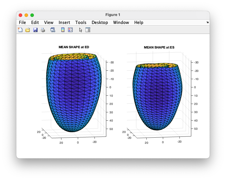

1.3 PCA calculation

% Let:
% S = n x 3m shape matrix
% mean_shape = the estimated mean shape
% output_folder is the folder to save the PCA components

% subtract each shape by the the mean_shape
S0 = S - repmat(mean_shape, size(S, 1), 1);

% calculate PCA
[coeff, score, latent, ~, explained, ~] = pca(S0);

%% some tests
ncomps = find(cumsum(explained)<99.9, 1, 'last');
fprintf(1, "Number of components covering 99.9%% = %g\n", ncomps);

figure;
plot(cumsum(explained(1:ncomps)));

%% save PCA
save(fullfile(output_folder, "PCA_coeff.mat"), "coeff");
save(fullfile(output_folder, "PCA_explained.mat"), "explained");
save(fullfile(output_folder, "PCA_latent.mat"), "latent");
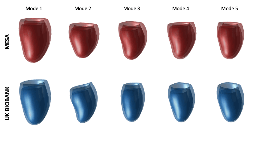
save(fullfile(output_folder, "PCA_score.mat"), "score");

The first 4 PCA modes of variations (±2.5 standard deviation from the mean shape) from MESA and UK Biobank studies used in the paper: